Clonal-aggregative multicellularity tuned by salinity in a choanoflagellate

A full description of the methods is provided in the Supplementary Information. All dilution percentages are v/v unless specified otherwise. No statistical methods were used to predetermine sample size. No blinding and randomization were used.

Cell strains and growth conditions

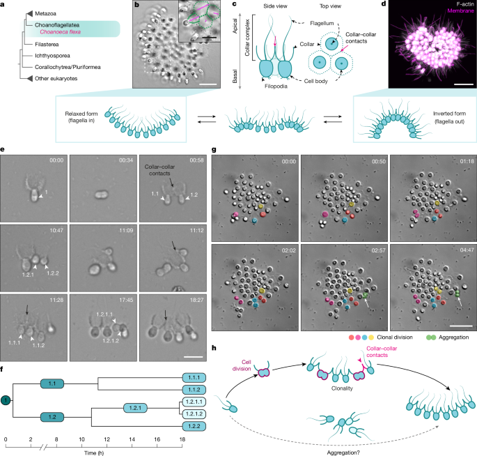
C. flexa clonal monoxenic cultures (strain ChoPs7, hereafter strain 1), established as described previously¹² from single-sheet cultures isolated near Boka Wandomi in Shete Boka National Park (the location reference is provided in Fig. 6a), were grown in 25 cm² tissue-culture-treated flasks (130189, Thermo Fisher Scientific) in either in 1% seawater complete (SWC) medium or 5% cereal grass medium 3 (CGM3) diluted in artificial seawater (ASW), following standard culture medium and culture protocols for choanoflagellates^12,25 with minor modifications (Supplementary Information).

Tracking cell division of single cells

The cell concentration of an exponentially growing ChoPs7 culture grown in SWC medium was estimated using a LUNA-II automated cell counter (LogosBiosystems). The culture was then diluted to 1 cell per µl in 5% SWC supplemented with 1% Halopseudomonas oceani resuspended food pellet (20 mg ml⁻¹ in ASW). A 1 µl aliquot of the diluted culture was pipetted onto the centre of a well in a black 96-well ibiTreat µ-plate (89626, Ibidi) and covered with 400 µl of Ibidi anti-evaporation oil (50051, Ibidi). The sample was imaged using a Plan-Apochromat ×20/0.8 M27 Zeiss objective on the Zeiss Axio Observer Z.1 inverted microscope, using tile scan mode to cover the entire droplet surface, Definite Focus and a ColorBand filter (FGL610, Thorlabs).

Time-lapse imaging of mixed clonal-aggregative multicellularity

Colonies from ChoPs7 cultures grown in CGM3 medium were transferred to a FluoroDish (FD35-100, World Precision Instruments) and incubated for 30 min to allow them to settle at the bottom of the dish. Colonies were imaged every 5 min by differential interference contrast (DIC) microscopy using a Plan-Apochromat ×63/1.4 oil-immersion Zeiss objective mounted on a Zeiss Observer Z.1 inverted microscope equipped with a Hamamatsu ORCA-Flash 4.0 V2 CMOS camera (C1140-22CU) in timelapse mode.

Aggregation dynamics over time

Two types of time-lapse videos of aggregation were generated: low-magnification overviews capturing a large number of cells imaged with a ×5 objective (Fig. 2b and Supplementary Video 4) and high-magnification, high-frequency videos of a smaller number of cells imaged with a ×63 objective to enable cell tracking (Fig. 2c,d and Supplementary Videos 5 and 6). The experiment was performed in four independent biological replicates (n = 4). For both types of experiments, 3 to 10 ml of dense ChoPs7 cultures were collected by centrifugation at 4,700g for 20 min at 4 °C, resuspended in supernatant and dissociated by vortexing for 30 s. The resulting cell suspension was transferred into a well of a Corning 96-well plate (13539050, Thermo Fisher scientific) for imaging and imaged overnight by DIC microscopy on the Zeiss Axio Observer Z.1 inverted microscope (details are provided in the Supplementary Information).

Staining and Airyscan imaging of aggregates at different stages

Approximately 10–20 ml of exponentially growing ChoPs7 cultures grown in SWC medium was collected by centrifugation at 3,300g for 15 min at room temperature and washed twice with 20 ml of 1× ASW. Cells were counted, seeded in 1 ml of ASW in a 24-well plate and incubated for 10 min, 30 min, 2 h, 6 h and 24 h at 25 °C. After incubation, 45 µl of cells was transferred into a 96-well plate (89626, Ibidi), fixed by adding ice-cold paraformaldehyde (PFA) (15710, Electron Microscopy Sciences) to a final concentration of 4%, permeabilized for 5 min with 0.1% Triton X-100 (A16046, Thermo Fisher Scientific) and stained with 1:1,000 FM 4-64X (F34653, Invitrogen) and 1:100 Alexa Fluor 488 Phalloidin (A12379, Invitrogen). The samples were imaged on the Zeiss Axio Observer Z1/7 microscope with LSM900 Airyscan 2.

Production, staining and imaging of dual-labelled chimeric aggregates

ChoPs7 cultures were collected as described above, resuspended in around 1 ml of ASW, dissociated by vortexing and divided into two 1.5 ml microcentrifuge tubes. Cells in each tube were stained 1:1,000 with either CellTrace CFSE (green; C34570, Thermo Fisher Scientific) or CellTrace Far Red (magenta; C34572, Thermo Fisher Scientific). Cells were collected again at 3,300g for 15 min at room temperature, washed once with 1 ml of 1% BSA in ASW, washed once more with 1 ml of ASW and resuspended in 500 µl of ASW. Cells were counted and mixed at a 1:1 ratio in 1 ml of SWC medium in a 24-well plate. Plates were incubated overnight at 25 °C, and non-mixed single-labelled populations were seeded in parallel as controls. After incubation, 100 µl of the sample was transferred into a 96-well plate, fixed with 4% PFA, permeabilized with 0.1% Triton X-100 and stained with 1:1,000 Alexa Fluor Plus 405 Phalloidin (A30104, Invitrogen). The samples were imaged using the LSM900 Airyscan 2 system as described above.

Quantification of aggregation in aphidicolin-treated cells

Chops7 cultures grown in CGM3 medium were treated overnight with aphidicolin or DMSO (drug vehicle control), dissociated by vortexing and transferred into an µ-Slide 8-Well chamber (80826, Ibidi). The samples were imaged every 30 min for 2 h on the Zeiss Observer Z.1 inverted microscope equipped with a Hamamatsu ORCA-Flash 4.0 V2 CMOS camera (C1140-22CU).

Aggregation of fixed versus live cells

ChoPs7 cultures were collected by centrifugation, resuspended in ASW, dissociated by vortexing, counted, vortexed again to ensure complete dissociation, seeded in a 24-well plate and immediately fixed with 4% PFA. Cells were then placed on an orbital shaker (Rotamax 120, Heidolph) at 50 rpm for 24 h at room temperature. Control plates containing live (non-fixed) cells and static (non-agitated) conditions were prepared in parallel. After 24 h, cells were imaged using transmitted light bright-field microscopy on a Zeiss Axio Observer Z.1 inverted microscope.

Field sampling

Fieldwork data were collected in Shete Boka National Park (12°22′5.718′ N, 69°06′56.916′ W) in Curaçao, in three independent expeditions during July–August 2023 and July–August 2024. The park spans nearly 10 km of rocky, wave-exposed coastline and contains approximately 10 pocket bays, or bokas.

Exped-A sampling and monitoring

For Exped-A, at least 10 ml of seawater was collected from n = 79 different splash pools (Sp1–Sp79) using 25 cm² tissue-culture-treated flasks along around 2 km of coastline. Fifteen of these splash pools (n = 15) were selected for daily monitoring of evaporation and refilling cycles over an 8-day time course. Each splash pool was uniquely identified using a physical tagging system and its GPS coordinates were recorded using an iPhone 12 Mini (Apple). A photograph of each splash pool and its surrounding environment was also taken using the same device. The following parameters were measured in situ: salinity using a refractometer (B07FQPFJGX (ASIN), Gain Express), temperature using a thermometer (B07CB8JG21 (ASIN), ThermoPro) and depth using measuring tape. Splash pool seawater or soil (in dry splash pools) were collected for rehydration experiments. The presence of sheets was visually assessed at the CARMABI biological station in Curaçao using the Leica DM IL LED inverted microscope equipped with the Nikon Z 50 camera. As controls, open sea salinity and temperature were measured in the bokas of Boka Wandomi and Boka Kalki.

Exped-B sampling

For Exped-B, a random-number generator was used to select a randomized sampling location between 150 m and 250 m upstream Boka Wandomi, avoiding sites that were previously sampled during Exped-A. At the selected location, an area measuring 10 m by 4 m was mapped and defined. All splash pools containing at least 5 ml of seawater within this area (n = 71) were collected and analysed as described above (M1–M77). New C. flexa strains (strain 2 and strain 3) were isolated from splash pools M44 and M60, respectively (see the ‘Manual isolation of sheets collected in the field’ section in the Supplementary Methods).

Exped-C sampling

For Exped-C, at least 10 ml of seawater was collected from n = 12 different splash pools (SpA–SpL) located near Boka Wandomi and Boka Pistol and analysed as described above. To maximize the likelihood of finding C. flexa sheets, the salinity of each splash pool was measured before sampling. Splash pools with salinity values within the permissive range for sheet occurrence (15–128 ppt) were selected for collection. The samples were later inspected using an inverted microscope to estimate C. flexa cell density based on the number of observed sheets (Supplementary Information).

Soil rehydration

A total of n = 32 soil samples was rehydrated across two independent fieldwork expeditions (Exped-A and Exped-C). Soil samples of n = 6 splash pools that underwent complete desiccation during Exped-A were scraped and collected daily for 8 days using a spatula into 25 cm² tissue-culture-treated flasks, ensuring that soil was sampled from multiple areas within each splash pool. Soil samples were rehydrated in the laboratory with 50–100 ml of sterile-filtered seawater collected from Boka Wandomi, adjusting the volume to reach a salinity of around 40 ppt. At least three independent rehydrations were performed for each sample. The presence of sheets was monitored daily during the next five days.

Soil samples of n = 26 additional splash pools (Soil1–Soil26) surveyed during Exped-C were collected, treated and monitored as described above with minor adjustments (Supplementary Information) as an independent replicate experiment.

Artificial evaporation

In total, 3 ml of dense ChoPs7 cells were seeded into four separate six-well plates (130184, Thermo Fisher Scientific) and transferred onto a grid inside a 30 °C incubator. One six-well plate was kept with its lid on (low-evaporation control), while the remaining plates were left uncovered (gradual-evaporation condition) over a 9-day time course. A plastic box (dimensions: 35.7 cm × 23.5 cm × 13.5 cm) was placed over the plates to allow for air exchange while minimizing contamination from airborne particles (Fig. 4a). At each timepoint, salinity was measured using a refractometer and a 100 µl sample was transferred into a 96-well plate for imaging on the Zeiss Axio Observer Z.1 inverted microscope and manual counting of cells in unicellular versus multicellular forms.

Cyst imaging under gradual evaporation

Cyst formation was monitored daily over a 4-day period using DIC microscopy on the Zeiss Observer Z.1 inverted microscope equipped with the Hamamatsu ORCA-Flash 4.0 V2 CMOS camera (C1140-22CU). Then, 200 ml of Chops7 cultures was transferred into a Bio-Assay Dish (240845, Thermo Fisher Scientific) and evaporated at 28 °C with the lid open for 4–6 h until the salinity reached 60 ppt. The temperature was increased to 29 °C and the lid was closed overnight to allow cells to adapt to the new salinity. The lid was partially reopened the next morning to resume gradual evaporation until the salinity reached 80 ppt; the lid was closed overnight, and the temperature was increased to 30 °C. The lid was reopened the next morning until the salinity reached 100–110 ppt. The culture was then maintained at that salinity with the lid closed for 24 h. On the morning of day 4, cells were imaged in a FluoroDish (FD35-100, World Precision Instruments).

Cyst F-actin and membrane staining

Cysts were produced using gradual evaporation at 30 °C to allow gradual evaporation (see the ‘Artificial evaporation experiment’ section in the Supplementary Methods), fixed with 4% PFA, transferred into a 96-well plate, permeabilized with 0.1% Triton X-100 and stained with 1:1,000 FM 4-64X, 1:100 Alexa Fluor 488 Phalloidin, and 1:100 Hoechst (H21486, Invitrogen). Samples were imaged using a Zeiss LSM900 Airyscan 2 as above.

Quantification of prey capture

A H. oceani food pellet (20 mg) resuspended in 1 ml ASW was stained with BactoView-Live Green (FITC) (40102, Biotium) at 4 µl ml⁻¹ and incubated for 30 min at room temperature in the dark, centrifuged at 2,750g for 5 min and resuspended in 1 ml ASW. In parallel, 200 µl of dense ChoPs7 cultures, or of single cells dissociated by vortexing, was transferred into 8-well chambers (80826, Ibidi). Then, 100 µl of stained bacteria diluted 1:20 in ASW was added to each well containing colonies or single cells. C. flexa was incubated with bacteria for 1 min before fixation with 4% PFA. After fixation, the samples were imaged using DIC and green fluorescence microscopy using the Zeiss Observer Z.1 microscope. The capture efficiency was calculated as the ratio between the number of bacteria attached to the collars of choanoflagellate cells to the total number of choanoflagellate cells in each image.

Normalized growth and efficiency of aggregation over 2 h

To calculate the normalized growth under the 1× and 2× salinity conditions (Fig. 5a), the growth rates obtained from experiment shown in Fig. 4m (see the ‘Growth quantification after gradual evaporation’ section in the Supplementary Methods) were normalized as follows:

Normalized growth = (growth rate)/(maximum growth rate across all conditions)

The efficiency of aggregation (E_a) for each individual experiment was calculated based on aggregation time lapses (see the ‘Time-lapse imaging of mixed clonal-aggregative multicellularity’ section above) at the 2 h timepoint as the ratio of the mean area of sheets obtained in that individual experiment over the maximal area observed under 2× salinity (Supplementary Information).

Efficiency of clonality and aggregation at different cell densities

Approximately 20 ml of dense ChoPs7 culture was collected and dissociated as described above. Then, 10², 10³, 10⁴ and 10⁵ cells were seeded in 1 ml of either 1× ASW or 2× ASW supplemented with 1% SWC and 0.5% H. oceani in a 24-well plate. Cells were incubated at 30 °C and imaged after 24 h, 48 h and 72 h incubation using bright-field microscopy on the Zeiss Axio Observer Z.1 microscope.

We defined the efficiency of aggregation (E_a) at a given cell density as the mean size reached at 24 h at that cell density under 2× salinity, normalized to the largest size measured at 2× salinity (across all cell densities) at 24 h. We defined the efficiency of clonality (E_c) as the additional growth allowed by cell division at 1× salinity relative to the aggregative baseline measured at 2× salinity (equations and technical details are provided in the Supplementary Information). As a control, we verified that our metrics for efficiency of aggregation and clonality were not saturated (Supplementary Information).

Staining and Airyscan imaging of aggregative and control sheets

For control sheets

Approximately 20 ml of dense ChoPs7 cells were collected and counted as above and seeded into 1 ml SWC medium in a 24-well plate at low density (~200 cells per ml) to favour clonal over aggregative formation of sheets. Cells were incubated for 3 days at 30 °C.

For aggregative sheets

Approximately 20 ml of dense ChoPs7 culture was collected, dissociated and counted, and 10⁵ cells were seeded in 1 ml of 2× ASW (with 1% SWC and 1% H. oceani) in a 24-well plate. Cells were incubated for 24 h at 30 °C.

Both types of sample were fixed with 4% PFA, stained with 1:1,000 FM 4-64X and 1:1,000 Alexa Fluor 488 Phalloidin as described above, and imaged using the Zeiss LSM900 Airyscan 2 microscope as described above. Cells per sheet were counted and collar–collar angles were quantified using Imaris v.9.9.1 (Bitplane, build 61122 for x64). Circularity was quantified using Fiji⁶¹ v.2.14.0/1.54f (Supplementary Information).

Light-regulated inversion in aggregative and control sheets

Aggregative and control sheets were produced as described above, transferred into a 96-well plate and imaged on the Leica Stellaris 5 confocal microscope with the HC PL FLUOTAR 10X/0.30 DRY objective in the FRAP mode. A white-light laser was used to create a 488 nm laser line with 1% intensity and a 633 nm laser line with 1% intensity. For light-to-dark stimulation, the 488 nm laser line was turned on during the pre- and post-bleaching frames and turned off during bleaching frames, while the 633 nm laser line remained continuously on. Bright-field images were acquired using the Trans PMT detector, and fluorescence signals were detected using two HyD type S, covering 495 nm–605 nm spectra for 488 nm excitation and 635 nm–745 nm spectra for 633 excitation, respectively. The imaging interval was around 0.19 s. Acquired images were exported in ‘ImageJ TIFF’ format using Leica Application Suite X.

Ten colonies from each replicate were subjected to light-to-dark transition to assess light-sensitive inversion behaviour (total of n = 60 sheets). For quantitative analysis, five representative colonies per condition were analysed to measure changes in colony area during inversion. Cell segmentation was performed on bright-field images using a custom-trained model of Cellpose (v.2.2.3)^62,63. The resulting colony masks were quantified using the label and regionprops_table functions from the measure module of the same package. The quantified area was normalized to the mean area of the first 20 frames before the light-to-dark transition and plotted using tidyverse (v.2.0.0) in R (v.4.1.1) and RStudio (v.2021.9.0.351).

Sequencing and assembly of the C. flexa reference genome

ChoPs cultures for genome sequencing and assembly were established by thawing a low-passage, previously reported C. flexa culture¹². Monoxenicity was established as previously described¹² by antibiotic treatment and addition of live H. oceani bacteria. The resulting ChoPs strain (ChoPs8) was grown to maximal density (around 1 × 10⁶ cells per ml) in 5% CGM3 medium. Bacteria were removed by spinning three times at 3,000g for 15 min, washing each time with 45 ml ASW. The final pellet was snap-frozen in liquid nitrogen and sent to Dovetail Genomics (Scotts Valley) for genomic DNA extraction, Omni-C+PacBio sequencing and genome assembly, which were performed by Dovetail Genomics staff using in-house protocols (details are provided in the Supplementary Information).

The genome of C. flexa was annotated using an integrated pipeline combining the results from several gene-calling algorithms with clues from C. flexa transcriptomic data and predicted proteomes from previously sequenced choanoflagellates⁶⁴. In total, 688,088 protein sequences were used as homology-based evidence for gene annotation. Protein sequences were aligned to the C. flexa genome using DIAMOND (v.2.1.8)⁶⁵ and exonerate (v.2.4.0)⁶⁶. DIAMOND identified 269,722 putative alignments and exonerate identified 2,679. Three gene prediction software packages were used to define 45,273 putative gene models. First, Augustus (v.3.3.2)⁶⁷ was run using Toxoplasma parameters, resulting in 6,822 high-quality predictions (>90% exon evidence) and 9,196 gene models without quality thresholding (15,676 total Augustus gene predictions). Second, SNAP⁶⁸, was trained using 194 eukaryotic BUSCO genes (v.2.0)⁶⁹ identified in the genome, yielding 15,083 gene models. Third, GlimmerHMM⁷⁰, trained on the same set of eukaryotic BUSCO genes, identified 14,172 gene models. All putative gene models were combined using a weighted consensus approach using the EvidenceModeler software⁷¹. This resulting set of 16,832 gene models was further filtered to remove sequences shorter than 50 amino acids in length, repetitive elements like transposons or spanned gaps. This filtering resulted in the removal of 186 gene models, and 16,646 total gene models remained. Workflow orchestration was performed using funannotate (v.1.8.16)⁷². The completeness of the gene models was assessed using BUSCO v.4.0.4, with the Eukaryota database of near-universally single-copy orthologous genes from OrthoDB (v.10)^73,74. This analysis revealed that the genome annotation is 83.6% complete. Lastly, tRNAs were identified in the genome assembly using tRNAscan-SE (v.2.0.9)⁷⁵, resulting in 237 tRNA models.

A final decontamination step was performed to remove putative bacterial contaminant sequences from H. oceani (NCBI accession: GCF_963677335.1), the bacterial food source used in C. flexa cultures. Three scaffolds were identified as probable contaminants by BLAST and removed from the final assembly (Supplementary Information).

The final C. flexa genome assembly spanned 56,404,751 base pairs (bp) across 528 scaffolds, with a GC content of 50.83%. The assembly N50 and L50 values were 1,302,044 bp and 16 scaffolds, respectively, and the largest scaffold measured 3,795,244 bp, indicating high assembly contiguity. The final genome annotation encoded 14,084 genes with an overall BUSCO completeness of 82.8%.

Whole-genome short-read sequencing of C. flexa strains isolated in the field

Cultures of strains 1, 2 and 3 were established after a single-cell bottleneck. gDNA was collected from dense cultures using either a lysis buffer coupled with ethanol and sodium acetate precipitation, or the Blood & Cell Culture DNA Mini Kit (13323, Qiagen) (Supplementary Information). All gDNA samples were shipped to Eurofins Genomics for INVIEW Resequencing (10 million paired-end reads, Illumina 150 bp sequencing). Paired-end reads were quality assessed and trimmed using FASTP (v.0.20.1)⁷⁶. Qualified reads were aligned to the C. flexa reference genome using BWA-MEM (v.0.7.17)⁷⁷. The mapped reads were converted to BAM format and sorted using Samtools (v.1.18)⁷⁸. Duplicate reads were marked using GATK (v.4.1.9.0)⁷⁹, and BAM files were indexed using Samtools v.1.18. Variant calling was performed using GATK HaplotypeCaller, applying different ploidy assumptions (ploidy = 1, 2 and 4) to detect potential polymorphisms across samples. The resulting variants were jointly genotyped for each ploidy condition using the GATK GenotypeGVCF function⁸⁰.

Phylogenomic tree construction

We realized that, although strains 2 and 3 seemed to be haploid, strain 1 (ChoPs7) exhibited a diploid-like pattern of allelic frequencies in scaffold_1, as assessed using ploidyNGS⁸¹. To accommodate samples with potentially differing ploidy levels, we used SNPs called under a diploid assumption and found homozygous across all samples for downstream analysis. Variants were filtered using BCFtools in Samtools (v.1.18)⁸² with the following criteria: quality score > 30, filtered read depth > 4, variant type = ‘SNP’, minimum and maximum allowed alleles = 2 and homozygous genotypes across all samples. The resulting VCF files were converted to PHYLIP format as input for IQ-TREE using the vcfR package⁸³ in R (v.4.1.1). A phylogenomic tree of all samples was constructed based on the identified SNPs using IQ-TREE (v.2.3.2) with the general time reversible (GTR) substitution model, gamma-distributed rate variation and ascertainment bias correction^84,85. The output tree structure was visualized using iTOL (v.6.9.1)⁸⁶.

Identification of polymorphic sites under putative diversifying selection

Coding sequences for each strain were inferred from the variant data using vcf2fasta (https://github.com/yeeus/vcf2fasta). Inferred coding sequences were programmatically checked across all reference sequences, and genes with incorrect inferences were removed from the analysis. Variants were jointly called for all strains using the GATK (v.4.1.9.0) and filtered according to the recommended parameters from the GATK team. The inferred coding sequences of each gene were checked for length integrity, retaining only those that were a multiple of 3, of equal length across strains and containing no gaps. Genes that did not satisfy those criteria were aligned using Clustal-omega (v.1.2.4), and those genes that introduced gaps that were not in multiples of 3 (causing frameshifts) were removed from the downstream analyses. To compare predicted protein sequences across strains, we computed the number of non-synonymous substitutions across the strains using Biopython (v.1.85)⁸⁷. The K_a/K_s ratio (that is, the dN/dS ratio) was calculated between strains to identify genes under putative diversifying selection. Moreover, we additionally computed sliding-window K_a/K_s ratios to capture localized signals of selection for subregions of each sequence, using KaKs_Calculator 2.0 with a window size = 114 bp and step size = 6 bp, and computed the K_a/K_s ratio using KaKs_Calculator 3.0 with the MYN method^88,89. We defined regions with K_a/K_s ratio > 2 for at least 30 bp as a high K_a/K_s region.

To explore functional enrichment, we computed InterPro signatures overlapping high K_a/K_s regions. InterPro signatures of the C. flexa predicted proteome were obtained using InterProScan (v.5.50-84.0)^90,91. The InterPro signature enrichment was performed using Fisher’s exact test in the base R stats package, comparing the frequency of each InterPro signature within versus outside high K_a/K_s regions. Enrichment analysis results were visualized using tidyverse (v.2.0.0)⁹².

Kin recognition experiments

Approximately 40 ml of dense cultures of strains 1, 2 and 3 were collected, washed and stained with CellTrace CFSE (green) and CellTrace Far Red (magenta) as described above. Green- and magenta-labelled single-cell populations from each strain were mixed in a 1:1 ratio (5 × 10³ cells of each colour) in 1 ml SWC medium in a 24-well plate and incubated overnight at 25 °C. After incubation, 100 µl of each sample were transferred into a 96-well plate and colonies were imaged in by DIC microscopy and epifluorescence microscopy on the Zeiss Axio Observer Z.1 inverted microscope. Green and magenta cells were manually counted, and kin recognition was quantified by calculating a segregation index between every pairwise strain combination defined in an previous study⁹³ (Supplementary Information).

Statistical analyses

The significance of differences in pairwise comparisons was tested using the non-parametric Mann–Whitney U-test. Shapiro–Wilk normality test and F-test were used to evaluate data normality and the differences in variances between conditions, respectively. All statistical analyses were performed in R Statistical Software (v.4.4.1)⁹⁴ using the base stats package (v.3.6.3).

Reporting summary

Further information on research design is available in the Nature Portfolio Reporting Summary linked to this article.