A sorghum pangenome reference improves global crop trait discovery

Plant material preparation and nucleic acid extractions

Young seedlings were grown in flat pans under healthy, pest-free and disease-free conditions until the first fully developed leaves emerged. To optimize DNA yield and quality, seedlings were dark-treated for 24–30 h under moist conditions. Tissue was collected by hand in small batches, cutting half an inch above the soil surface and immediately flash-freezing in liquid nitrogen within 1 min of excision. Approximately 50 g of tissue was collected in this manner, stored in pre-labelled freezer-quality ziplock bags at –80 °C and kept frozen until extraction. DNA was extracted from young tissue using a previously published protocol⁵⁴ with minor modifications. Flash-frozen young leaves were ground to a fine powder in a frozen mortar with liquid nitrogen followed by gentle extraction in 2% CTAB buffer (including proteinase K, PVP-40 and β-mercaptoethanol) for 30 min to 1 h at 50 °C. After centrifugation, the supernatant was gently extracted twice with 24:1 chloroform and isoamyl alcohol. The aqueous phase was transferred to a new tube and one-tenth volume 3 M sodium acetate was added, gently mixed and DNA was precipitated with isopropanol. DNA precipitate was collected by centrifugation, washed with 70% ethanol, air dried for 5–10 min and dissolved thoroughly in an elution buffer at room temperature followed by RNAse treatment. DNA purity was measured with Nanodrop, and the DNA concentration was measured using a Qubit HS kit (Invitrogen). DNA size was validated using a Femto Pulse system (Agilent).

We also grew three biological replicates of the reference genotypes (see Supplementary Data 12 for phenotype data and Supplementary Data 13 for original photographs without the backgrounds removed) and sampled them at key developmental stages and organ types for transcriptome assembly and genome annotation (sample and data collection were performed by the team at Donald Danforth Plant Science Center in 2020). For the 29 diverse pangenome reference members and BTx623 (excluding, BTx642, Wray and RTx430), tissues were collected from greenhouse-grown sorghum plants maintained under controlled environmental conditions. For each replicate, tissues from multiple plants were pooled when individual tissue quantity was insufficient. Six tissue types were represented in the samples. (1) Approximately half-inch sections of stem tissue were excised from each internode and nodal region of the same stem at 60 days after planting (DAP), immediately frozen in liquid nitrogen and pooled to generate composite stem samples. (2) At 28 DAP, the youngest fully expanded leaf was collected and subdivided into tip, base, midrib and sheath segments, which were pooled to represent the composite leaf sample. (3) Entire primary and crown root systems were harvested at 28 DAP, gently rinsed with water to remove adhering soil and pooled per replicate. (4) Developing inflorescences were collected at both heading and anthesis to capture pre-pollination and post-pollination reproductive stages. Whole inflorescences were excised, flash-frozen and pooled across plants. (5) Developing grain was sampled at 5 DAP, 20 DAP and at the black layer stage to represent early, mid and late seed development, respectively. (6) Whole seedlings were collected at 12 DAP under well-watered (100% field capacity (FC)) and water-stressed (45% FC) conditions. Water stress was initiated 5 DAP, and both shoot and root tissues were harvested and pooled at 12 DAP. In addition to these developmental-stage collections, time-course sampling was conducted for two representative genotypes, PI660565 and PI276816, to capture early vegetative dynamics. For each line, three biological replicates were collected at 10, 17, 21, 25 and 31 DAP. At each time point, leaf and stem tissues were collected following the same procedures described above. Immediately after collection, all tissues were flash-frozen in liquid nitrogen and stored at –80 °C until RNA extraction. Tissue collection for Wray and for BTx642 and RTx430 (as previously detailed²⁶) generally followed the above protocol, but with some differences in the types of tissues.

Genome assembly

Long-read sequencing technology, as used in the construction of our pangenome reference assemblies, has improved the resolution of repetitive regions and closed gaps in other complex genomes^55,56. Although the quality and contiguity of our pangenome assemblies are consistent, the input data depth, sequencing technology, bioinformatic methods available and sequencing read characteristics necessitated some differences in computational genome assembly strategy. Here we provide a summary of the basic methods (see Supplementary Note 2 for a full description of genome assembly methods for each reference genome).

The majority of the pangenome sequences were generated by assembling PACBIO CLR reads with CANU (v.1.8)⁵⁷, whereas five accessions (PI156178, RTx430, BTx642 and PI565121) were assembled with MECAT (v.1.4)⁵⁸, and one accession (Wray) was generated using PACBIO HiFi data assembled with HiFiAsm+HIC (v.16.1)⁵⁹. All sequencing was conducted at the HudsonAlpha Institute for Biotechnology and the Department of Energy (DOE) Joint Genome Institute. All assemblies were subsequently polished using ARROW (v.2.1)⁶⁰, except BTx623 and Wray, which were polished using RACON (v.1.14)⁶¹. A combination of 32,400 syntenic markers (unique, non-repetitive, nonoverlapping 1.0-kb sequences from BTx642) and 12,641 annotated genes from BTx623 were used to identify misjoins in the assembly. Contigs were then ordered, oriented and assembled into ten chromosomes after examining syntenic marker and gene alignment positions on the polished assemblies. Each chromosome join was padded with 10,000 Ns. Contigs terminating in significant telomeric sequence were identified using the (TTTAGGG)n repeat, and care was taken to make sure that they were properly oriented in the production assembly. Chromosomes were numbered using BTx623 V3 naming convention. The remaining scaffolds were screened against bacterial proteins, organelle sequences, and GenBank non-redundant datasets and removed if found to be a contaminant. Chloroplast and mitochondrial genomes were generated using the OatK pipeline (v.1.0)⁶². Homozygous SNPs and indels were corrected to match the consensus call from Illumina fragment reads (2 × 150, 400 bp insert) by aligning the reads using bwa-mem (v.0.7.17-r1188)⁶³ and identifying homozygous SNPs and indels with the UnifiedGenotyper tool in GATK (v.3.6-0-g89b7209)⁶⁴.

Genome annotation

Genome annotation was performed using the pipeline developed by the DOE Joint Genome Institute and Phytozome⁶⁵. As methodological considerations can substantially affect estimates of protein-coding gene PAVs³⁰, each pangenome member underwent two rounds of gene prediction. In the first round, gene models were independently predicted for each genome followed by the propagation of these predictions across the entire pangenome in the second round.

In the initial round, transcript assemblies were generated from 2 × 150 bp stranded paired-end Illumina RNA sequencing reads (Supplementary Table 2) using PERTRAN (as previously described in detail⁶⁶) for genome-guided assembly via GSNAP (v.2013-09-30)⁶⁷, followed by splice graph construction, alignment validation and correction. PacBio Iso-Seq CCS reads, when available, were corrected and collapsed using a GMAP-based pipeline⁶⁷ to refine alignments, correct splice junctions and cluster alignments when their intron (or introns) matches if spliced or 95% similar if it was a single exon. Final transcript assemblies were produced using PASA (v.2.0.2)⁶⁸, integrating RNA sequencing assemblies, corrected CCS reads and Sanger ESTs. A species-specific repeat library was built from BTx623 V3 using RepeatModeler (v.open1.0.11)⁶⁹. Repeats were functionally analysed with InterProScan (v.5.47-82.0)⁷⁰, incorporating Pfam⁷¹ and PANTHER⁷² databases, and those with significant hits to protein-coding domains were excluded. Genomes were soft-masked using RepeatMasker (v.open1.0.11)⁶⁹ with the curated repeat library. Gene loci were identified using transcript assembly and EXONERATE (v.2.4.0)⁷³ alignments of proteins from Arabidopsis, soybean, poplar, Aquilegia, grape, rice, Setaria viridis, Brachypodium, Panicum hallii, pineapple, Acorus americanus and Swiss-Prot (2020_06) to the repeat soft-masked genomes, with up to 2,000-bp extension on both ends unless extending into another locus on the same strand. Gene models were predicted using FGENESH+ (v.3.1.0)⁷⁴, FGENESH_EST, EXONERATE, PASA assembly ORFs and AUGUSTUS (v.3.1.0)⁷⁵ trained on high-confidence PASA assembly open reading frames with intron hints from RNA sequencing alignments. Candidate models were selected based on EST and protein support and penalized for repeat overlaps. PASA refinement added UTRs, corrected splicing and incorporated alternative isoforms. Cscore (BLASTP score ratio and protein coverage) was computed for PASA-refined proteins. Transcripts were retained if Cscore and coverage was ≥0.5 or supported by ESTs; those with >20% CDS-repeat overlap required a Cscore ≥ 0.9 and ≥ 70% coverage. Models with >30% TE domain overlap (Pfam) were excluded.

In the second round, each genome was hard-masked with its high-confidence gene models (supported by transcriptome and homology evidence). BLASTX and EXONERATE were used to predict new gene models by projecting high-confidence models from other pangenome members onto the hard-masked assemblies. Predicted models were retained if they showed stronger homology support than existing models and were not contradicted by transcript evidence, or if no first-round model existed at that locus. Incomplete gene models, which had low homology support without full transcriptome support, or short single exon genes (<300 bp CDS) without protein domain or good expression were manually excluded.

Pangenome graph construction and exploration

A pangenome graph was constructed for each chromosome using Minigraph-Cactus and default settings (v.2.9.3)⁷⁶ with the BTx623 V5 genome as the primary reference. Clipped chromosome graphs were merged and prepared for visualization using vg (v.1.59.0)⁷⁷. We used ODGI (v.0.9.0)⁷⁸ to inspect representation of each genome across the graph and sequenceTubeMap (v.0.1.0)⁷⁹ to visualize variation in genomic regions of interest. For the dhurrin BGC and SH1 loci, we further processed this graph with vg and vcfwave (vcflib v.1.0.10)⁸⁰ to reduce allelic complexity and retain only variants ≥5 kb and ≥1 kb in length, respectively.

Comparative genomics

Gene families were calculated with OrthoFinder (v.2.5.5)⁸¹ and parsed with GENESPACE (v.1.3.1)⁸² to create saturation curves. Synteny maps were created using DEEPSPACE (v.0.1.0, github.com/jtlovell/DEEPSPACE), which aligns and tracks the positions of windowed sequence alignments and quickly visualizes large-scale SVs. SyRI (v1.6.3)⁸³ was used for pairwise variant detection from whole-genome alignments via minimap2 (v.2.22-r1101)⁸⁴. Pangenome graph saturation curves were calculated with Panacus⁸⁵.

DNA re-sequencing and variant detection

A total of 2,145 diversity samples (n = 1,984 unique genotypes + redundant + polishing) were re-sequenced at a median coverage of 43.39× (range 1.96–364.18) (Supplementary Data 3). The samples were sequenced using Illumina HiSeq X10 and Illumina NovaSeq 6000 paired-end sequencing (2 × 150 bp) at the HudsonAlpha Institute for Biotechnology and the Joint Genome Institute. To account for different library sizes, reads were downsampled to ≤50× coverage.

SNPs and short indels were called by aligning Illumina reads to the BTx623 V5 reference with bwa mem⁶³. The resulting .bam file was filtered for duplicates using Picard (http://broadinstitute.github.io/picard) and realigned around indels using GATK (v.3.056)⁶⁴. Multisample SNP calling was done using SAMtools (v.1.7) mpileup⁸⁶ and Varscan (v.2.4.089)⁸⁷ with a minimum coverage of eight and a minimum alternate allele count of four. Genotypes were called using a binomial test. Variants within 25 bp of a 24-mer repeat were removed from further analyses. For most analyses, only SNPs with minor allele frequencies (MAFs) of >0.001 were retained, which resulted in 36,061,325 SNPs at a coverage depth between 8× and 500×. Phasing was performed using SHAPEIT (v.3)⁸⁸.

Pangenome-based genotyping

To project patterns of observable diversity in the pangenome assemblies to the broader whole-genome resequencing panel, we applied k-mer-based genotyping to SH1 and the dhurrin BGC locus. In brief, the k-mer genotyping methodology extracts ancestry-informative k-mers^34,35 for genomic regions of interest and counts exact matches of these k-mers in Illumina sequencing libraries. In this instance we used 80-mers that were globally single-copy (but could be duplicated locally) within individual references and absent in at least one member of the pangenome. This methodology is analogous to a k-mer-based GWAS⁸⁹, but instead of testing for genome-wide associations using accession-derived k-mer PAV, it aggregates k-mers from pangenome references that are unique to and diagnostic of a haplotype in a predefined region of interest (ROI).

The pipeline proceeded as follows. First, each reference genome was individually converted into k-mers; each k-mer and its frequency in the assembly were stored in a hash table. Any non-adjacent multicopy k-mers were flagged to be ignored during downstream analyses. Second, individual reference hashes were combined in a single hash (‘main hash’), and the flags were updated so that only single copy k-mers among all considered references were used downstream (for example, a single-copy k-mer in reference A was ignored if it was multicopy in reference B). To isolate k-mers that were useful for genotyping a ROI (for example, the SH1 or dhurrin BGC loci), the orthologous region from each reference was extracted (from either from the pangenome graph or best alignment bounds) using minimap2 (ref. ⁸⁴). Steps 1 and 2 above were repeated on the subsetted fasta files, which generated a combined subsetted hash that contained local single-copy sequences from all ROI orthologues across the pangenome. Third, to ensure that the ROI local single-copy markers did not occur elsewhere in the genome, which would prevent their use as a genotyping marker, the combined ROI hash was intersected with the main genome hash, and flags were updated so that any non-single copy k-mers were ignored when genotyping (‘genotyping hash’). The total number of diagnostic k-mers (globally single copy and not common to all pangenome reference members) used in the genotyping approach was 6,533 for the SH1 locus and 139,866 for the dhurrin BGC locus. Fourth, Illumina libraries were genotyped by searching for all k-mers in the genotyping hash and counting their frequencies. At this point, counts were either merged into a single matrix for de novo clustering (for example, dhurrin BGC locus), or binned based on a priori clusters (for example, SH1 locus) based on the local haplotype structure at the region of interest. De novo clustering as used for k-mer genotyping the dhurrin BGC locus operated on a binary matrix of n × m (k-mer presence/absence × Illumina libraries), where k-mer frequencies greater than one were considered present. Clusters were visualized in principal component space and coloured by clustering as defined by partitioning around medoids (PAMs) of pairwise Jaccard distances among reference libraries. A priori clustering was used for k-mer genotyping the SH1 locus as the per cent match to diagnostic k-mers in each bin. Illumina library haplotypes were then assigned to a SH1 cluster based on majority match to haplotype bins.

To generate the dot plots in Fig. 3, the position of SH1 was queried from the pangenome graph by ‘vg find‘, returning intervals the following nodes in the native genome coordinate systems on chromosome 1: BTx623: 12,398,577–12,400,453 bp, 12,400,454–12,401,958 bp, 12,401,959–12,404,976 bp; MN2014: 12,177,214–12,179,090 bp, 12,179,091–12,181,356 bp, 12,181,357–12,182,863 bp, 12,182,864–12,185,897 bp; RTx430: 12,088,419–12,090,291 bp, 12,090,292–12,092,556 bp, 12,092,557–12,094,061 bp, 12,094,062–12,101,908 bp, 12,101,909–12,104,942 bp. These contiguous sequence blocks (BTx623 12,398,577–12,404,976 bp; MN2014: 12,177,214–12,185,897 bp; RTx430: 12,088,419–12,104,942 bp) were converted to 80-mers and aligned to the RTx430 genomic interval with minimap2 (parameters = -r80,800 -O6,26 -e2,1 -B4 -f0.0001 -p0.5 -N100 -k19 -w12 -g160 -F800 -t8 -A1 -U50,500 -no-long-join -rmq=no -n1 -m0 -frag=yes), retaining the primary (mapq = 60) hits or those hits within 1 bp of the number of mismatches in the primary alignment. The aligned k-mers were binned into those among the diagnostic 80-mers (see above) or those that are not diagnostic and coloured according to the genome to which they are unique.

Diversity panel source material

The sorghum diversity panel used in this study comprised 1,984 unique accessions sourced from structured diversity panels and curated regional collections. These lines spanned Africa, Asia and the Americas and represented both landraces and breeding lines, thereby providing broad coverage of genetic, phenotypic and geographic variation of sorghum and 10 discrete genetic resources or populations. (1) CASP: 82 lines from a 648-line association panel previously described⁹⁰, which was developed for trait mapping under field and drought conditions. (2) Biomass Association Panel (BAP): 390 accessions representing biomass-related diversity across sorghum botanical types and global regions⁹¹. The panel is widely used in bioenergy trait mapping, and 375 of the BAP accessions are included in this study. (3) Sorghum Association Panel (SAP): 377 genotyped accessions developed by USDA-ARS and collaborators⁹², which represents all five major sorghum races and is widely used in GWAS. A total of 328 SAP accessions are included in this study. (4) TERRA MEPP: represents a wide range of traits relevant to field-based high-throughput phenotyping. These lines were selected to enable trait discovery under environmental variation⁹³. (5) Purdue Inbred Calibration Set: a set of accessions with which emphasize improving traits related to drought, cold tolerance, striga resistance, nutritional quality and biomass potential. These lines have played a central part in UAV-based remote-sensing studies that integrate hyperspectral and LiDAR data with marker profiles, which underscores their relevance in phenomics–genomics research^94,95. (6) Georeferenced Panel: 529 lines including 166 accessions from the BAP, 133 African accessions from the WRS and an additional 230 accessions from NPGS-GRIN, selected to maximize spatial sampling. Georeference coordinates were sourced from Genesys using ICRISAT IDs (IS numbers) and cross-referenced with NPGS-GRIN IDs (PI numbers) for GRIN accessions. (7) World Reference Set (WRS): 383 accessions⁹⁶, which capture broad allelic diversity, including all five major cultivated races and their intermediates. The set reflects extensive geographical coverage, spanning central and eastern Africa to Western Africa, South Asia and East Asia, with significant representation in domesticated morphotypes rather than strict race categories. Our study includes 381 of these 383 accessions, thereby preserving nearly the full scope of genetic and geographic diversity defined therein. (8) West African Sorghum Association Panel (WASAP): a 756-member diversity panel contributed by national programmes in Mali, Senegal, Togo and Niger to represent West African landraces and regionally adapted breeding lines. (9) Ethiopian Institute of Agricultural Research (EIAR): a regional collection developed and curated by EIAR to capture the exceptional diversity of Ethiopian highland sorghum. These accessions include seed-increased landraces and genotyped lines selected for local adaptation. (10) BC-NAM Parents: 37 founder accessions from a West and Central African Backcross Nested Association Mapping (WCA-BCNAM) population, as previously partially detailed⁹⁷. These lines were selected for adaptation traits and crossed with three elite recurrent parents from the region, yielding 3,901 BC-NAM lines. The founders were chosen to maximize genetic diversity in plant height, flowering time and environmental response across agro-ecologies varying in photoperiod, rainfall, temperature and fertility⁹⁷. This panel structure reflects global efforts to unite diverse germplasm for climate-aware trait discovery and genomic breeding.

Passport data collection and curation

Passport data—including botanical classification, breeding improvement status, country of origin and geographical coordinates—were compiled from multiple sources: the GRIN-Global database, Genesis Global, the ICRISAT Sorghum Passport dataset and previously published studies^93,98. Records were cross-referenced to identify and resolve discrepancies across datasets. In cases where inconsistencies could not be reconciled, both conflicting metadata entries were retained and included in the final metadata.

Population genetics

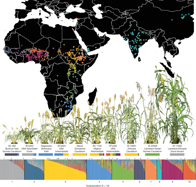
We applied ADMIXTURE (v.1.3.0)⁹⁹ using default settings to n = 1,984 unique genotypes of non-duplicated sequencing libraries. To generate an approximately independent set of markers, we removed variants with MAF < 0.05, more than 50% missingness, and applied LD-based pruning with a window size of 50 SNPs, step size of 5 SNPs and a r² threshold of 0.5 in PLINK (v.1.90b6.12)¹⁰⁰. After filtering, we randomly selected 100,000 SNPs to estimate the optimal K of ancestral groups (optimal K ≈ 10, see Supplementary Note 4 and Supplementary Fig. 3 for details). For the remainder of population genetic analyses, we retained n = 433 samples georeferenced to the African continent that were designated as landraces, cultivars or wild strains and missed a genotype call in <15% sites. To select sites that captured dynamics of population structure, we selected putatively neutral and unlinked variants using bcftools (v.1.9)¹⁰¹ with the following filtering parameters: invariant sites and sites with strand bias in variant-supporting reads (>90%) were removed. We required all retained variants to be synonymous, have a genotype call in at least 95% of individuals sampled and a MAF ≥ 0.01. Filtered genotypes were imputed with beagle (v5.4) ¹⁰² and variant effects annotated with SnpEff (v5.1d)¹⁰³. We further LD-pruned the remaining SNPs in PLINK using 50-SNP windows with a variance inflation factor (VIF) of 2 (VIF = 1/(1 – R²), where R² is the multiple correlation coefficient for a SNP being regressed on all other SNPs simultaneously, PLINK documentation), resulting in a set of 33,823 neutral LD-pruned SNPs.

We used these 33,823 SNPs to estimate effective migration surfaces in fast estimation of effective migration surfaces (FEEMS⁴¹). We ran separate analyses for the African continental axes (north–south and east–west). For each independent run of FEEMS we optimized the smoothing regularization parameter (λ) and utilized the optimal lambda for each analysis. Node and edge positions and weights were exported and formatted for plotting in R. To describe patterns in allele frequency change at neutral sites capturing dynamics of population structure, we again used the set of 33,823 imputed, neutral and LD-pruned SNPs. Georeferenced samples (n = 433) were grouped into populations by averaging allele frequencies of samples georeferenced to the same latitude and longitude (rounded to 3 decimal places, around 100 m), which resulted in 343 populations comprising 1 and 13 individuals (mean = 1.26). We estimated scale-specific genome-wide turnover by modelling the allele frequency change with wavelet transformations at 15 scales, spaced along a log sequence from the 0.1st to 99th percentile of distances between sites: 24 km, 35 km, 49 km, 69 km, 98 km, 139 km, 197 km, 278 km, 394 km, 558 km, 790 km, 1,119 km, 1,584 km, 2,242 km and 3,174 km. We compared patterns of sorghum wavelet-transformed allele frequencies to previous estimates in A. thaliana⁴⁰, and to an analysis of published pearl millet genotype data¹⁰⁴. Population-averaged pearl millet genotypes¹⁰⁴ were filtered to remove any markers with missing data, which retained 138,948 markers from 174 populations. We conducted the scale-specific wavelet analysis at 15 scales, spaced along a log sequence from the 0.1st to 99th percentile of distances between sites: 33 km, 44 km, 59 km, 79 km, 105 km, 140 km, 187 km, 249 km, 332 km, 443 km, 591 km, 788 km, 1,051 km, 1,400 km and 1,867km.

Following previously described methods¹⁰⁵, we also used wavelet transformations of our sorghum genotypes to determine outlier loci with more rapid spatial allele frequency change compared with the overall distribution, which represent loci that may be important in adaptation. We used 5,615,029 SNPs filtered for MAF > 0.01 and heterozygosity <0.9 (which are probably representative of genotyping errors). The top 1,000 outliers from each chromosome at each spatial scale were used in downstream analyses, including a gene ontology enrichment using topGO (v.2.42.0), an R Bioconductor package.

Using the same set of SNPs, we identified putative selective sweeps using normalized xpnsl (v.1.3.0)⁴⁴, grouping georeferenced populations into geographical regions using PAM and comparing individuals from high-drought prevalence sites to individuals from low-drought prevalence sites in each of five geographical regions (a sixth region included only high-drought prevalence sites and was excluded). We retained all sites with normalized scores above the critical threshold and converted runs of sites into blocks. We then quantified pairwise base-pair overlap of xpnsl extended haplotypes reciprocally between all geographical regions. We determined whether overlap was greater than expected by chance by comparing the observed overlap to the overlap of permuted genomic blocks, significance testing relative to 1,000 permutations. We compared the amount of haplotype overlap using paired t-tests for each geographical region.

Assignment of landraces to climate-based clusters

Following previously described methods¹⁰⁶, the Cycles agroecosystem model was used to characterize variables representative of stage-specific water stress (vegetative and reproductive) for the point of origin for n = 326 sorghum landrace accessions. Cycles is a process-based multiyear and multispecies agroecosystem model that simulates biophysical and management practices in cropping systems^107,108 to simulate crop growth. All simulations were carried out using Cycles (v.0.13.0; https://github.com/PSUmodeling/Cycles). The crop description file defines the physiological and management parameters that control the growth and harvest of crops used in the simulation. We used the base Cycles sorghumMS parameters from the default crop description file. The management (operation) file defines the daily management operations to be used in a simulated crop rotation. We activated conditional planting where Cycles ‘plants’ a simulated crop once certain soil moisture and temperature levels are satisfied in a window of planting dates. We turned on the automatic nitrogen fertilization option and set planting density to 67% so that stress observed in model outputs was due entirely to climatic factors. To approximate the climate conditions the sorghum accessions were adapted to, we simulated plant growth using weather data from 1970 to 1989, 10 years before and after the average collection year. Daily weather files at one-quarter degree resolution that overlapped with at least one of our georeferenced accessions and for years included in the simulation were fetched from the meteorological data source Global Land Data Assimilation System (GLDAS¹⁰⁹) using the script LDAS-forcing.py sourced from GitHub (https://github.com/shiyuning/LDAS-forcing). Soil physical parameters describing the average soil characteristics and land-use type of each landrace accession point of origin were obtained from the ISRIC SoilGrids global database¹¹⁰ via the HydroTerre data system^111,112,113. Using model outputs and for each landrace accession, we extracted integrative environmental variables representative of stress when in the vegetative and reproductive phase. Accessions were clustered into two groups (low-drought and high-drought prevalence) using k-means clustering implemented in the R stats package. As additional georeferenced landraces were added to the diversity set (n = 107), cluster membership was predicted using a feedforward artificial neural network (ANN) implemented in the R package neuralnet (v1.44.2, https://CRAN.R-project.org/package=neuralnet). The ANN used bioclimatic predictors from the WorldClim 2.1 dataset (1970–2000)¹¹⁴, interpolated at 10 arcmin resolution (around 340 km² per pixel). Input variables included mean temperature of the driest quarter (MTDQ), mean temperature of the warmest quarter (MTWQ), precipitation of the wettest month (PWM), precipitation seasonality (PS), precipitation of the driest quarter (PDQ) and precipitation of the warmest quarter (PWQ).

Dhurrin phenotyping

To evaluate variation in dhurrin concentration and HCNp among diverse sorghum germplasm, we conducted a single time-point phenotypic analysis using accessions sourced from the USDA Germplasm Resources Information Network (GRIN). All accessions were grown under controlled conditions at the Colorado State University Plant Growth Facilities (HCNp was analysed during first planting in autumn 2022 and second planting in spring 2023; dhurrin was analysed in spring 2023). A completely randomized block design was implemented with two replicates per accession. Four plants per accession were sown in 11.4 l pots containing Pro-Mix HP supplemented with one tablespoon of Osmocote fertilizer. Accessions were evaluated across two separate plantings, each containing two replicate blocks. In each block, individual plants were grown and subsequently sampled for trait assessment. Sampling for HCNp was performed at the seedling stage (3–4-leaf stage) and again at the early vegetative stage (7–8-leaf stage), with tissues from the youngest fully expanded leaf collected from each plant. Dhurrin was estimated at the seedling stage for only a single replicate in one of the plantings. All plant tissue samples were processed individually and randomly assigned to plates to control for technical variation. Blocks were nested in plantings to account for potential variation.

Plates were kept on ice during sample collection and stored at –20 °C. Cyantesmo test strips (Macherey–Nagel) were cut to fit each plate, applied across alternating rows and sealed with Axygen microplate film (Corning). Pressure was applied to each plate to limit gas transfer between wells, and plates were incubated at –35 °C for 20 min. Strips were removed from the plates and imaged with a flatbed scanner. Images were converted to the CIELAB colour space and ROIs were defined around each blue reaction area, with each ROI representing a single sample. ROIs were thresholded on the b* (0–128; ranging from blue to yellow) and L* (128–255; lightness) channels. Blue intensity was calculated on a per pixel basis by subtracting the pixel L* value from 255. Blue intensity values in a ROI were summed and the resulting value was normalized by the ROI area to quantify HCNp.

Dhurrin concentration was quantified using ultrahigh-performance liquid chromatography coupled with tandem mass spectrometry (UHPLC–MS/MS). Leaf samples were harvested, dried at 60 °C for approximately 3 days and ground using a Bead Ruptor Elite tissue grinder (6 cycles at 4 m s^–1, 15 s each, with 10-s breaks). A 100 mg aliquot of ground tissue was extracted with 750 μl of 50% methanol (v/v methanol and diH₂O), incubated in a 75 °C water bath for 15 min, cooled to room temperature (10–15 min) and supplemented with an additional 750 μl of 50% methanol. Samples were centrifuged at 11,000 rpm for 5 min. A 30 μl aliquot of the supernatant was diluted with 270 μl of LC–MS-grade water (final 5% methanol, dilution factor 0.15 ml mg^–1), transferred to a 2 ml glass HPLC vial and stored at –80 °C. Quality control (QC) was maintained using pooled QC samples prepared from aliquots of individual extracts. Blank extractions were also included. Samples were stored at –80 °C until analysis.

One microlitre of extract was injected into a LX50 UHPLC system (PerkinElmer) equipped with a 20-µl sample loop (partial loop injection mode). Chromatographic separation was performed using an Acquity UPLC HSS T3 column (1 × 50 mm, 1.8 µm; Waters) maintained at 45 °C. The mobile phases consisted of water with 0.1% formic acid (A) and 100% acetonitrile (B). The elution gradient started at 1% B for 0.5 min, ramped linearly to 99% B over 4.5 min, returned to 1% B at 5.2 min and was followed by a 2.8 min re-equilibration, for a total run time of 8 min. The flow rate was set to 400 µl min^–1. Detection was carried out on a PerkinElmer QSight 420 triple quadrupole mass spectrometer equipped with an electrospray ionization (ESI) source operating in positive mode and selected reaction monitoring (SRM). The optimized SRM transitions for dhurrin were based on an authentic standard: Q1/Q3 = 333.9/144.9 for quantification and 333.9/184.9 for qualification. Source parameters were as follows: drying gas temperature at 120 °C, hot-surface induced desolvation (HSID) temperature at 200 °C, electrospray voltage at 5,000 V and nebulizer gas flow at 350. MS acquisition was scheduled around a retention time of 1.14 min with 1 min time windows. The dwell time for each transition was 100 ms. Data acquisition and processing were performed using Simplicity 3Q software (v.3.0, PerkinElmer). Quantification was based on standard curves generated from authentic dhurrin standards using linear regression. Concentrations are expressed as µg g^–1 fresh weight, adjusted for sample weight and dilution factors.

Whole plant phenotyping

For full details, see Supplementary Note 5. In brief, field-based measurements were collected in 2023 and 2024 across multiple locations captured key agronomic traits, including plant height, flowering time, panicle architecture and yield components, with data separated by replication and site to enable genotype × environment interaction analyses. Phenotyping was conducted by the team at Donald Danforth Plant Science Center in 2023 and 2024. High-resolution temporal vegetation indices, extracted from drone-based overhead imagery (Supplementary Table 4), further characterized canopy development and biomass dynamics over the growing season. Controlled-environment phenotyping complemented field trials to quantify WUE and drought response under well-watered and water-limited conditions using automated indoor imaging systems. Growth curve data across treatments enabled classification of genotypes by their drought response strategies, including early vigour and maintenance of growth under stress. Greenhouse-based evaluations provided additional trait measurements under standardized conditions, including early vigour and developmental timing (Supplementary Data 12). Visual documentation of phenotype diversity was collected across environments, including a curated set of representative field and greenhouse images for each genotype.

Environmental gradients associated with genomic variation in sorghum georeferenced lines

We used redundancy analysis (RDA) implemented with linear regression and principal component analysis to examine how environmental gradients explain genome-wide SNP variation among 443 sorghum landraces and to partition the variance in genomic diversity attributable to different sets of environmental variables. RDA combines multiple regression with ordination to identify the environmental dimensions that best account for multilocus genetic structure and to quantify the proportion of total genomic variation explained by the environment. Environmental variables included climatic factors, elevation, water balance, radiation, soil physicochemical properties and risk of striga. All variables were standardized before analysis, and samples with missing data for any variable were excluded. Genotype matrices were centred and regressed on the standardized environmental matrix; principal components of the fitted values defined the constrained axes (RDA axes) and their variance contributions. The overall model fit, expressed as adjusted r² = 0.1948, indicated that the selected environmental variables jointly explained about 19.5% of genome-wide SNP variation.

Dhurrin and cyanide genome-wide association

GWAS were performed using a linear mixed model implemented in GEMMA (v.0.98.3)¹¹⁵. Only directly called genotypes were used; no imputation was performed. Variants were filtered to retain those with a MAF ≥ 0.05, resulting in 8963567 SNPs and short indels. For each trait, association statistics were computed using the Wald test. Markers with missing or undefined P values were excluded from downstream analyses. The filtered results were used to generate Manhattan plots and to assess overlap with a priori candidate genes. Significance was determined by FDR-correcting raw P values using the Benjamini–Hochberg method, implemented in the R internal function p.adjust.

In silico ligand docking of tyrosine to CYP79A1 protein variants

To evaluate the impact of sequence variants on the binding affinity of CYP79A1 for its substrate tyrosine, in silico ligand docking was performed using SwissDock (https://www.swissdock.ch). Homology models in Protein Data Bank (PDB) format of wild-type and mutant CYP79A1 proteins were generated using SWISS-MODEL (https://swissmodel.expasy.org) using FASTA sequences as input and subsequently oriented in the endoplasmic reticulum (ER) membrane using the PPM3.0 server of the Orientation of Proteins in Membranes (OPM) database (https://opm.phar.umich.edu/ppm_server). The resulting OPM-oriented PDB files were manually cleaned to remove water molecules and extraneous heteroatoms. The MOL2 file for the substrate l-tyrosine was downloaded from the PubChem database and used as the ligand for docking. PDB files of CYP79A1 containing either an alanine (A211) or valine (V211) at position 211, oriented in the membrane as described above, were used as the target structures. Each docking run was performed under default settings, using the ‘Docking with AutoDock Vina’ option to scan for potential ligand-binding regions. SwissDock returned a series of clusters, each associated with an estimated binding free energy (ΔG) in kcal mol^–1. The binding affinity of tyrosine to each CYP79A1 variant was compared by identifying the lowest predicted ΔG value across all clusters. More negative ΔG values were interpreted as indicative of stronger substrate binding. Predicted docking structures were visualized using PyMOL (https://www.pymol.org/) to confirm that the substrate tyrosine localized in the active site of each protein model and to generate the renderings shown in Extended Data Fig. 5b,c.

Dhurrin BGC cis-element analysis

To test whether intergenic variants associated with seedling dhurrin content reside in regulatory regions with accessible chromatin and potential transcription factor (TF) binding sites, the Plant PAN 4.0 and SorghumBase¹¹⁶ resources were used. Genomic coordinates of intergenic variants in the BGC were examined using the Ensembl Plants genome browser hosted through SorghumBase to assess whether they overlapped with known accessible chromatin regions. Specifically, the accessible chromatin region track derived from ATAC–seq profiling of 7-day-old S. bicolor leaf tissue, as previously published¹¹⁷, was used, which provides a high-resolution map of chromatin accessibility across the genome. To test whether these intergenic variants also overlapped with putative TF binding sites, each variant sequence was extracted along with 10 bp of flanking sequence on both sides. These sequences were input into PlantPAN (v.4.0), a promoter and cis-element prediction tool that integrates binding site data from multiple plant-specific motif databases. Only predicted TF-binding sites that directly overlapped the variant position were retained for downstream analysis, under the assumption that such overlap may indicate mutation of a functional cis-regulatory element. To maximize confidence in predicted TF–DNA interactions, only hits that included both a known TF family and a corresponding Arabidopsis gene identifier were considered for downstream analysis.

Statistics and reproducibility

Sequencing and genotyping of all Illumina libraries was performed once. In cases when this resulted in duplicated genotypes, we avoided pseudo-replication by only retaining the library with higher depth of uniquely mapping reads for each duplicated genotype. Phenotyping campaigns were spatially and temporally replicated as described in Supplementary Note 5 (with details regarding phenotype data collection and processing).

Reporting summary

Further information on research design is available in the Nature Portfolio Reporting Summary linked to this article.